Analyzing a Cloud-Native IVT Zarr for Atmospheric Rivers
Description
This notebook shows how to authenticate with HydroShare and stream a cloud-native Zarr (~40 GB) of Integrated Vapor Transport (IVT) derived from the CESM2 Large Ensemble (LENS2). The full collection (~1.9 PB, NetCDF) is hosted by the NSF Research Data Archive (dataset d651056). In August 2024, we extracted a ~40 GB IVT subset from the legacy NCAR archive and republished it on HydroShare in Zarr format. Using HydroShare’s S3-compatible endpoint with xarray+dask, we perform time/space subsetting and detect atmospheric rivers (ARs) with the common IVT ≥ 250 kg/m/s threshold, then assign AR categories based on joint intensity and duration. We also compute an “AR degree” metric, defined as event-integrated IVT (the sum of IVT over an event’s duration; IVT × days), as a simple indicator of event severity.
Software Requirements
This notebook has been tested using Python v3.11.8 using the following library versions:
dask>=2025.7.0
xarray>=2024.2.0
geopandas>=1.1.1
h5netcdf>=1.6.4
hvplot>=0.11.3
requests>=2.32.2
rioxarray>=0.19.0
s3fs>=2025.5.1
numpy>=2.3.1
cftime>=1.6.4
folium>=0.20.0
Environment Setup: Imports & Dask (Cluster/Client)
import os
import sys
import cftime
import dask
import folium
import hvplot.xarray
from dask.distributed import Client
import s3fs
import numpy as np
import xarray as xr
from pathlib import Path
import cartopy.crs as ccrs
import cartopy.feature as cfeature
import matplotlib.pyplot as plt
import requests
import importlib.util
from getpass import getpass
from hsclient import HydroShare
from hsmodels.schemas.fields import BoxCoverage, PointCoverage, PeriodCoverage
from hsmodels.schemas.fields import AwardInfo
from datetime import datetime
def is_installed(package_name):
    return importlib.util.find_spec(package_name) is not None
import ARUtils
print("h5netcdf installed:", is_installed("h5netcdf"))
print("h5py installed:", is_installed("h5py"))
# Check if the required packages are installedC:\Users\AbnerBogan\anaconda3\envs\ciroh-devcon-2026-workshop-hydroinformatics\Lib\site-packages\rdflib\plugin.py:111: UserWarning: pkg_resources is deprecated as an API. See https://setuptools.pypa.io/en/latest/pkg_resources.html. The pkg_resources package is slated for removal as early as 2025-11-30. Refrain from using this package or pin to Setuptools<81.
from pkg_resources import iter_entry_points
h5netcdf installed: True
h5py installed: True
# use a try accept loop so we only instantiate the client
# if it doesn't already exist.
try:
    print(client.dashboard_link)
except:
    # The client should be customized to your workstation resources.
    # This is configured for a "Large" instance on ciroh.awi.2i2c.cloud
    # client = Client()
    client = Client(n_workers=4, threads_per_worker=2, memory_limit="3GB")
    print(client.dashboard_link)

dask.config.set({'array.slicing.split_large_chunks': True})
C:\Users\AbnerBogan\anaconda3\envs\ciroh-devcon-2026-workshop-hydroinformatics\Lib\site-packages\distributed\node.py:188: UserWarning: Port 8787 is already in use.
Perhaps you already have a cluster running?
Hosting the HTTP server on port 59308 instead
  warnings.warn(
http://127.0.0.1:59308/status
<dask.config.set at 0x29c58e381d0>Authenticate to HydroShare & Configure S3FS
The following cells first obtain S3 credentials from the HydroShare API, initialize s3fs for the HydroShare S3 endpoint, and find the exact bucket and key prefix for the resource, then combine them to build s3_path for listin/reading the Zarr store.
The Zarr store contained in the HydroShare resource below is part of a larger collection of CESM2 LENS model outputs on AWS maintained by NCAR.
Authenticate your HydroShare account and identify the HydroShare resource containing the IVT data:
# sign into HydroShare
username = "abogan" # <- Make sure to change your HS username
password = getpass('Enter your password: ')
resource_id = "53effa6f532b43a5972daa5336932224"
Enter your password: ········
Access the HydroShare API endpoint to create and retrieve temporary S3 credentials for an authenticated HydroShare user:
# create an S3 access key and secret key for the authenticated user
response = requests.post(f"https://hydroshare.org/hsapi/user/service/accounts/s3/", auth=(username, password))
response_json = response.json()
access_key = response_json['access_key']
secret_key = response_json['secret_key']
Run the next cell to create a connection to the HydroShare S3 bucket using the s3fs library. s3fs provides a filesystem-like interface to S3, making it easy to list, read, and write files as if they were on your local machine. For more information, refer to the s3fs documentation.
# create a filesystem-like client for S3
s3 = s3fs.S3FileSystem(key=access_key,
                       secret=secret_key,
                       endpoint_url='https://s3.hydroshare.org')
# get the s3_path for the resource_id
response = requests.get(f"https://hydroshare.org/hsapi/resource/s3/{resource_id}/", auth=(username, password))
response_json = response.json()
s3_path = f"{response_json['bucket']}/{response_json['prefix']}"
s3.ls(s3_path)['igarousi/53effa6f532b43a5972daa5336932224/data/contents/ivt.zarr']For pushing files back to HydroShare later in this notebook, we can also authenticate with HydroShare directly with the hsclient library. Here, you can also define your HydroShare user object by going to your profile in HydroShare and extracting the user ID from the URL of your profile (e.g., for Abner Bogan’s profile https://www.hydroshare.org/user/24566/, his user ID is 24566).
hs = HydroShare(username, password)

user_id = 1183
hs_user = hs.user(user_id)
Open the Integrated Vapor Transport (IVT) Zarr Store Lazily
A Zarr store is not a single file, but actually:
a directory-like collection
contains many chunk files + metadata
more like a smart reference system describing where the data live and how to compute with them later
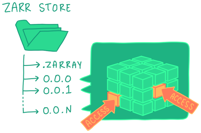
Max Jones, Development Seed
As we will see, the IVT Zarr store is large. Before we retrieve the numerical data arrays, we use a method called “lazy loading” to read only the metadata, coordinates, and structure by using xarray and dask. After doing this the data are still sitting remotely in HydroShare. Lazy loading avoids unnecessary downloading of large quantites of data while still accessing the information we need to subset the dataset at a location and time period of interest.
filename='ivt.zarr'
# create interface between remote S3 access and filesystem-style access
mapper = s3.get_mapper(f"{s3_path.rstrip('/')}/{filename}")

# read metadata, variables/dimensions/chuncks, build lazy array objects
# (`consolidated=True` reads the zarr metadata from the combined metadata file)
ds = xr.open_zarr(mapper, consolidated=True)

# you'll see this object is lazy Dask arrays, not a fully loaded numpy.ndarray
print(type(ds.IVT.data))
<class 'dask.array.core.Array'>
The Zarr dataset behaves like a directory tree of chunk files and metadata objects stored in cloud object storage.
Inspect the Mapper Object directly to see some of the contents of the Zarr store:
list(mapper.keys())[:20]['.zattrs',
'.zgroup',
'.zmetadata',
'IVT/.zarray',
'IVT/.zattrs',
'IVT/0.0.0',
'IVT/1.0.0',
'IVT/10.0.0',
'IVT/100.0.0',
'IVT/101.0.0',
'IVT/102.0.0',
'IVT/103.0.0',
'IVT/104.0.0',
'IVT/105.0.0',
'IVT/106.0.0',
'IVT/107.0.0',
'IVT/108.0.0',
'IVT/109.0.0',
'IVT/11.0.0',
'IVT/110.0.0']Inspect the xarray.Dataset to see the information we can access with Lazy Loading:
dsExpanding the icon for Data variables:IVT above reveals a table with important information about the Zarr store and the Dask chunking. This summary table shows that a ~38 GB multidimensional dataset is being represented lazily as 367 independently accessible ~105 MB chunks. This allows Dask to stream only the needed pieces instead of loading the entire dataset into memory.
Check the IVT dataset chunk sizes.
→ This zarr store is partitoned only temporally, not spatially. This means that each chunk contains 1000 timesteps for the FULL model domain.
# print(ds.IVT.chunks)
print(ds.IVT.chunksizes)
Frozen({'time': (1000, 1000, 1000, 1000, 1000, 1000, 1000, 1000, 1000, 1000, 1000, 1000, 1000, 1000, 1000, 1000, 1000, 1000, 1000, 1000, 1000, 1000, 1000, 1000, 1000, 1000, 1000, 1000, 1000, 1000, 1000, 1000, 1000, 1000, 1000, 1000, 1000, 1000, 1000, 1000, 1000, 1000, 1000, 1000, 1000, 1000, 1000, 1000, 1000, 1000, 1000, 1000, 1000, 1000, 1000, 1000, 1000, 1000, 1000, 1000, 1000, 1000, 1000, 1000, 1000, 1000, 1000, 1000, 1000, 1000, 1000, 1000, 1000, 1000, 1000, 1000, 1000, 1000, 1000, 1000, 1000, 1000, 1000, 1000, 1000, 1000, 1000, 1000, 1000, 1000, 1000, 1000, 1000, 1000, 1000, 1000, 1000, 1000, 1000, 1000, 1000, 1000, 1000, 1000, 1000, 1000, 1000, 1000, 1000, 1000, 1000, 1000, 1000, 1000, 1000, 1000, 1000, 1000, 1000, 1000, 1000, 1000, 1000, 1000, 1000, 1000, 1000, 1000, 1000, 1000, 1000, 1000, 1000, 1000, 1000, 1000, 1000, 1000, 1000, 1000, 1000, 1000, 1000, 1000, 1000, 1000, 1000, 1000, 1000, 1000, 1000, 1000, 1000, 1000, 1000, 1000, 1000, 1000, 1000, 1000, 1000, 1000, 1000, 1000, 1000, 1000, 1000, 1000, 1000, 1000, 1000, 1000, 1000, 1000, 1000, 1000, 1000, 1000, 1000, 1000, 1000, 1000, 1000, 1000, 1000, 1000, 1000, 1000, 1000, 1000, 1000, 1000, 1000, 1000, 1000, 1000, 1000, 1000, 1000, 1000, 1000, 1000, 1000, 1000, 1000, 1000, 1000, 1000, 1000, 1000, 1000, 1000, 1000, 1000, 1000, 1000, 1000, 1000, 1000, 1000, 1000, 1000, 1000, 1000, 1000, 1000, 1000, 1000, 1000, 1000, 1000, 1000, 1000, 1000, 1000, 1000, 1000, 1000, 1000, 1000, 1000, 1000, 1000, 1000, 1000, 1000, 1000, 1000, 1000, 1000, 1000, 1000, 1000, 1000, 1000, 1000, 1000, 1000, 1000, 1000, 1000, 1000, 1000, 1000, 1000, 1000, 1000, 1000, 1000, 1000, 1000, 1000, 1000, 1000, 1000, 1000, 1000, 1000, 1000, 1000, 1000, 1000, 1000, 1000, 1000, 1000, 1000, 1000, 1000, 1000, 1000, 1000, 1000, 1000, 1000, 1000, 1000, 1000, 1000, 1000, 1000, 1000, 1000, 1000, 1000, 1000, 1000, 1000, 1000, 1000, 1000, 1000, 1000, 1000, 1000, 1000, 1000, 1000, 1000, 1000, 1000, 1000, 1000, 1000, 1000, 1000, 1000, 1000, 1000, 1000, 1000, 1000, 1000, 1000, 1000, 1000, 1000, 1000, 1000, 1000, 1000, 1000, 1000, 1000, 1000, 1000, 1000, 1000, 1000, 1000, 1000, 1000, 1000, 1000, 1000, 1000, 1000, 1000, 1000, 1000, 1000, 1000, 1000, 1000, 1000, 1000, 462), 'lat': (192,), 'lon': (288,)})
Check file size. Zarr chunks are compressed on disk. HydroShare shows the compressed total (e.g., 24 GiB). ds.nbytes reports the uncompressed size of all arrays in the dataset, i.e., what it would take in RAM if loaded.
print(f'Variable size: {ds.nbytes/1e9:.1f} GB')
print('Number of years in one file:', round(ds.time.shape[0]/4/365))
Variable size: 40.5 GB
Number of years in one file: 251
The time coordinate in this dataset is not strictly monotonic increasing, which can break label-based slicing, resampling, and merges. First, check it with the custom function time_order_report() and then fix the order:
def time_order_report(ds: xr.Dataset, dim: str = "time"):
    idx = ds.indexes.get(dim)
    if idx is None:
        raise KeyError(f"No index found for '{dim}'.")
    print(
        f"{dim}: monotonic↑={idx.is_monotonic_increasing}, "
        f"monotonic↓={idx.is_monotonic_decreasing}, "
        f"unique={idx.is_unique}, "
        f"length={len(idx)}"
    )
    return idx

# Example usage
idx = time_order_report(ds)
idx
time: monotonic↑=False, monotonic↓=False, unique=False, length=366462
CFTimeIndex([1970-01-01 00:00:00, 1970-01-01 06:00:00, 1970-01-01 12:00:00,
             1970-01-01 18:00:00, 1970-01-02 00:00:00, 1970-01-02 06:00:00,
             1970-01-02 12:00:00, 1970-01-02 18:00:00, 1970-01-03 00:00:00,
             1970-01-03 06:00:00,
             ...
             2100-12-29 18:00:00, 2100-12-30 00:00:00, 2100-12-30 06:00:00,
             2100-12-30 12:00:00, 2100-12-30 18:00:00, 2100-12-31 00:00:00,
             2100-12-31 06:00:00, 2100-12-31 12:00:00, 2100-12-31 18:00:00,
             2101-01-01 00:00:00],
            dtype='object', length=366462, calendar='noleap', freq=None)
# If not strictly increasing or not unique, fix it:
ds = ds.sortby("time")
# Re-check
_ = time_order_report(ds)
print(f"Start: {ds.time.min().values}")
print(f"End: {ds.time.max().values}")time: monotonic↑=True, monotonic↓=False, unique=False, length=366462
Start: 1850-01-01 00:00:00
End: 2101-01-01 00:00:00
Also, the time axis is a CFTimeIndex, i.e., it uses cftime date types for non-Gregorian calendars (e.g., noleap, 360_day). Many plotting and pandas/xarray functions work best with standard NumPy datetimes, so we convert to proleptic_gregorian (and drop cftime) before plotting:
# Convert to proleptic_gregorian and drop cftime (requires modern xarray)
ds = ds.convert_calendar("proleptic_gregorian", use_cftime=False)

# If there are duplicate timestamps, drop them first (optional but helpful)
if ds.get_index("time").has_duplicates:
ds = ds.sel(time=~ds.get_index("time").duplicated())Note: This conversion will drop timestamps that do not exist in the Gregorian calendar (e.g., Feb 29 in noleap).
Subset to a Location and Period of Interest
Display the full model domain
Before we subset the IVT data for a location, let’s take a look at the spatial area contained in the Zarr store (hint: it’s very large!)
# isolate and load in only one timestep of the Zarr store
ivt0 = ds.IVT.isel(time=0).compute()

# use xarray to inspect metadata attributes of the loaded data
print(ivt0.name)
print(ivt0.attrs)

# compute the bounds of the full model domain (i.e., the Zarr store dataset)
bounds = [
    [float(ds.lat.min()), float(ds.lon.min())],
    [float(ds.lat.max()), float(ds.lon.max())]
]
IVT
{'long_name': 'Total (vertically integrated) vapor transport', 'units': 'kg/m/s'}
Plot the full domain extent of the IVT data for a single timestep. Here, we are using the Python package cartopy and accessing a coastline shapefile (ax.coastlines()) from the Natural Earth public domain dataset repository.
# plot the full extent of the IVT data for one timestep
fig = plt.figure(figsize=(12,8))
ax = plt.axes(projection=ccrs.PlateCarree())

ivt0.plot(
    ax=ax,
    transform=ccrs.PlateCarree(),
    cmap='viridis',
    cbar_kwargs={"shrink": 0.6}
)

ax.coastlines()
ax.set_title(f"IVT at timestep {ds.time.isel(time=0).values}")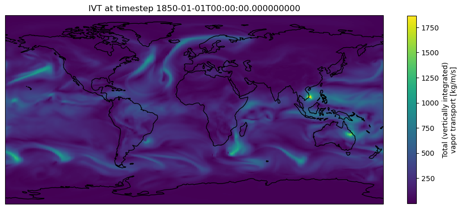
The cartopy download warning appears the first time you download the coastline shapefiles from Natural Earth because these files are retrieved on demand rather than bundled locally with the Python package.
This is conceptually similar to the cloud-native Zarr workflow in this notebook: xarray + Dask access only the specific IVT Zarr metadata and data chunks needed for the current computation or visualization, rather than downloading the full dataset upfront.
Subset IVT for location and time of interest
Next, we can subset the IVT for a given location and time period. By default we have selected Bodega Bay (38.3332° N, 123.0481° W), a region frequently impacted by wintertime atmospheric rivers—major drivers of seasonal precipitation and flooding across the Pacific Northwest and Northern California (see https://
point_name = "Bodega Bay"
start_date="1970-01-01"
end_date="2009-12-31"
lat = 38.
lon = -123.125
m = folium.Map(location=[lat, lon], zoom_start=10)
folium.CircleMarker([lat, lon], radius=6, color="red", fill=True, fill_opacity=0.8,
popup=f"Lat {lat:.4f}, Lon {lon:.4f}").add_to(m)
mSimilar to the on-demand access of the cartopy visualization above, the folium package used here is generating an interactive Leaflet web map and instructs the browser to request only the needed map tiles without downloading the entire map file locally.
Lazily subset the IVT Zarr store for the time period and point location defined above:
ds_point = ds.sel(time=slice(start_date, end_date)).sel(lat=lat, lon=lon+360., method='nearest').IVT
ds_pointLoad the subsetted data.
→ This step is where we are actually triggering the retrieval of the selected data chunk into memory!
%%time
ds_point = ds_point.load()
ds_point.shape

# save the dataframe to CSV
ds_point.to_dataframe().to_csv("ivt_timeseries.csv")
CPU times: total: 25.3 s
Wall time: 2min 36s
Create a timeseries of IVT at the selected lat/lon point:
p = (ds_point.hvplot(label='IVT', color='black', line_dash='dashed', line_width=1)
).opts(
    width=900, height=400, show_grid=True, tools=['hover']
)

p Select a set of grid cells around the lat/lon point that cover Bodega Bay, CA (38.3332° N, 123.0481° W).
# the nearest index for the lat/lon provided above
ilon = list(ds.lon.values).index(ds.sel(lon=lon+360., method='nearest').lon)
ilat = list(ds.lat.values).index(ds.sel(lat=lat, method='nearest').lat)

cell_buffer = 10
# subset these data to include cells above and below this lat/lon
ds_box = ds.sel(time=slice(start_date, end_date)).isel(lat=range(ilat-cell_buffer, ilat+cell_buffer),
                  lon=range(ilon-cell_buffer, ilon+cell_buffer)).IVT

ds_box = ds_box.to_dataset()
Load the subsetted grid cells (and selected data chunks) into memory:
%%time
ds_box = ds_box.load()
CPU times: total: 23.5 s
Wall time: 2min 6s
Plot the IVT data for these cells at time=0 to visualize our domain:
fig, ax = plt.subplots()
ax.set_xticks([])
ax.set_yticks([])
ax = plt.axes(projection=ccrs.PlateCarree())

#add coastlines
ax.coastlines()

#add lat lon grids
gl = ax.gridlines(draw_labels=True, color='lightgrey', alpha=0.5, linestyle='--')
gl.xlabels_bottom = False
gl.ylabels_right = False

plot = ds_box.isel(time=0).IVT.plot(label='',
                         add_labels=False,
                         add_colorbar=False,
                         xticks=None,
                         yticks=None)

# add custom colorbar inside the figure
cbar_ax = fig.add_axes([0.99, 0.25, 0.02, 0.5])  # [left, bottom, width, height] in figure coords
cbar = plt.colorbar(plot, cax=cbar_ax)
cbar.set_label('IVT (kg m⁻¹ s⁻¹)')

ax.plot(lon+360., lat,
        marker='o', color='red', markersize=8,
        transform=ccrs.PlateCarree())

plt.show()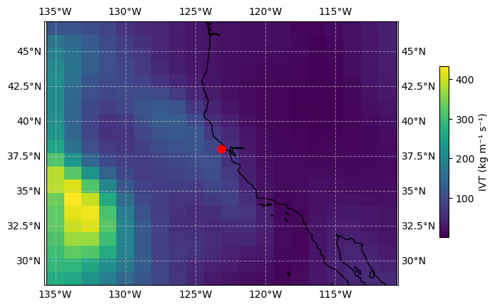
ds_boxds_box.chunksFrozen({})Identify Atmospheric River Events
To identify atmospheric rivers, we first flag periods where IVT ≥ 250 kg/m/s, a common screening threshold for AR conditions (Ralph et al., 2019). We then classify AR strength into Categories 1–5 using the Ralph et al. (2019) scale, which combines peak IVT and event duration. Lower categories indicate weaker ARs, while higher categories indicate extreme/exceptional events. This workflow is implemented in our Python utility module ARUtils.py.
# # Ensure time is a single chunk (so events aren’t broken across chunks)
# ds_box = ds_box.chunk({"time": -1})
# ds_box.chunks
Assign an index to each group of timesteps that meet AR conditions
ds_box['AR_INDEX'] = xr.apply_ufunc(
    ARUtils.identify_ar_events,
    ds_box.IVT,
    input_core_dims=[["time"]],
    output_core_dims=[["time"]],
    vectorize=True,
    dask='parallelized',
    dask_gufunc_kwargs={'allow_rechunk': True},
)
Compute the duration for each AR event
ds_box['AR_DURATION'] = xr.apply_ufunc(
    ARUtils.compute_ar_durations,
    ds_box.AR_INDEX,
    input_core_dims=[["time"]],
    output_core_dims=[["time"]],
    vectorize=True,
    dask='parallelized',
    dask_gufunc_kwargs={'allow_rechunk': True},
)
Compute the category (1-5) for each AR event
ds_box['AR_CATEGORY'] = xr.apply_ufunc(
    ARUtils.compute_ar_category,
    ds_box.AR_INDEX,
    ds_box.AR_DURATION,
    ds_box.IVT,
    input_core_dims=[["time"],["time"],["time"]],
    output_core_dims=[["time"]],
    vectorize=True,
    dask='parallelized',
    dask_gufunc_kwargs={'allow_rechunk': True},
)
Compute the probability of each AR event occurring
res = xr.apply_ufunc(
    ARUtils.compute_ar_probability,
    ds_box.AR_INDEX,
    ds_box.AR_CATEGORY,
    input_core_dims=[["time"],["time"]],
    output_core_dims=[['category']],
    # output_sizes={'category': 5},
    output_dtypes=[float],
    vectorize=True,
    dask='parallelized',
    dask_gufunc_kwargs={'allow_rechunk': True,
                        'output_sizes': {'category': 5}},
)

# Add the category dimension (from 1 to 5)
res = res.assign_coords(category=np.arange(1, 6))

# add the newly computed probabilty back to the original dataset
ds = ds.assign(AR_PROBABILITY=res)
Compute the magnitude of each AR event.
ds_box['AR_DEGREE'] = xr.apply_ufunc(
    ARUtils.compute_ar_degree,
    ds_box.IVT,
    ds_box.AR_DURATION,
    ds_box.AR_INDEX,
    input_core_dims=[["time"],["time"],["time"]],
    output_core_dims=[['time']],
    output_dtypes=[float],
    vectorize=True,
    dask='parallelized',
    dask_gufunc_kwargs={'allow_rechunk': True},
)
Plot Computed AR Category
Mean Atmospheric Rivers category through the record of data. Let’s first build contour plots of mean AR_CATEGORY for each decade in our dataset using cartopy.
year = ds_box["time"].dt.year
decade = np.floor(year / 10) * 10
ds_box = ds_box.assign_coords({'decade':decade})
ds_decade = ds_box.where(ds_box.AR_CATEGORY > 0) \
.AR_CATEGORY \
.groupby('decade') \
.mean(dim='time').compute()fig, ax = plt.subplots(nrows=2, ncols=2,
subplot_kw={'projection': ccrs.PlateCarree()},
figsize=(10,8),
layout='constrained')
axes = ax.flatten()
for i in range(0, len(ds_decade.decade)):
axes[i].coastlines();
axes[i].gridlines(draw_labels=True, color='lightgrey', alpha=0.5, linestyle='--');
# created grid and contour plots.
d_plot = ds_decade.isel(decade=i).plot(label='',
add_labels=False,
add_colorbar=False,
ax=axes[i])
c_plot = ds_decade.isel(decade=i).plot.contour(add_labels=True,
add_colorbar=False,
colors='white',
ax=axes[i])
axes[i].clabel(c_plot)
st = int(ds_decade.decade[i].item())
et = st + 9
axes[i].set_title(f'{st} - {et}')
fig.colorbar(d_plot, ax=ax[:, 1], shrink=0.8);
fig.suptitle('Mean Decadal AR Category');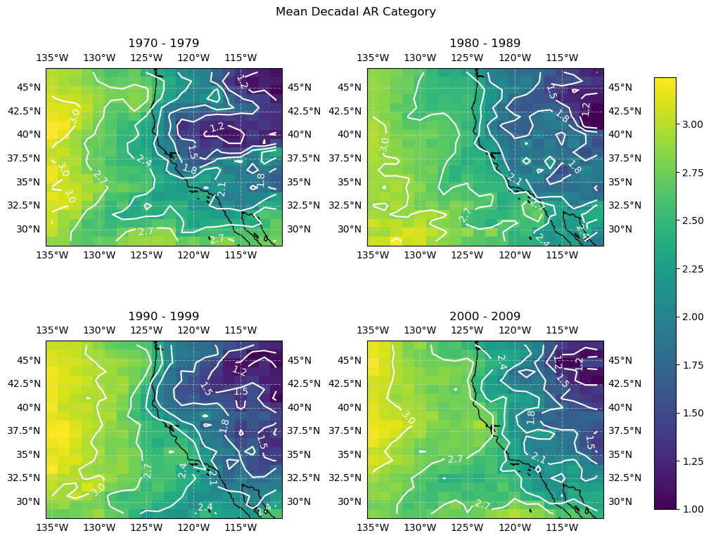
Build contour plots of mean AR_DEGREE for each decade in our dataset.
ds_decade = ds_box.where(ds_box.AR_CATEGORY > 0) \
            .AR_DEGREE \
            .groupby('decade') \
            .mean(dim='time').compute()
import matplotlib.ticker as ticker
fig, ax = plt.subplots(nrows=2, ncols=2,
subplot_kw={'projection': ccrs.PlateCarree()},
figsize=(10,8),
layout='constrained')
axes = ax.flatten()
for i in range(0, len(ds_decade.decade)):
axes[i].coastlines();
axes[i].gridlines(draw_labels=True, color='lightgrey', alpha=0.5, linestyle='--');
# created grid and contour plots.
d_plot = ds_decade.isel(decade=i).plot(label='',
add_labels=False,
add_colorbar=False,
ax=axes[i])
c_plot = ds_decade.isel(decade=i).plot.contour(add_labels=True,
add_colorbar=False,
colors='white',
ax=axes[i])
# custom formatting function for contour labels on the maps
def fmt_func(value):
return f'{value:.0e}'
axes[i].clabel(c_plot, inline=True, fontsize=10, fmt=fmt_func)
st = int(ds_decade.decade[i].item())
et = st + 9
axes[i].set_title(f'{st} - {et}')
fig.colorbar(d_plot, ax=ax[:, 1], shrink=0.8);
fig.suptitle('Mean Decadal AR Degree');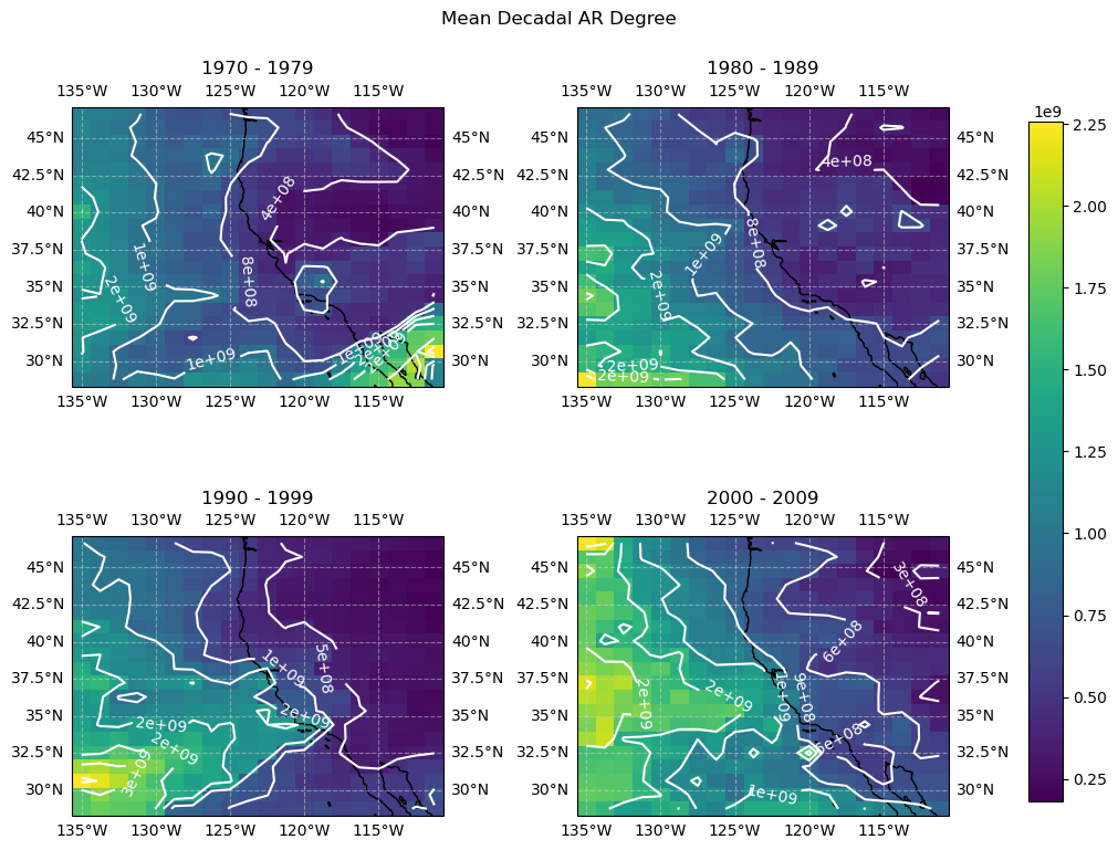
🎉 Save the Mean Decadal AR Degree Figure for our HydroShare Resource!
fig.savefig(
    "mean_decadal_ar_degree.png",
    dpi=150,
    bbox_inches="tight"
)
Push data back into HydroShare
Now that we have extracted, analyzed and visualized our data of interest, we can push the data back to HydroShare in a new resource through the Python client for the HydroShare API called hsclient.
Create a New Empty Resource
The following code can be used to create a new, empty resource within which you can create content and metadata.It also creates an in-memory object representation of that resource in your local environmment that you can then manipulate with further code.
# Create the new, empty resource
new_resource = hs.create()

# Get the HydroShare identifier for the new resource
res_identifier = new_resource.resource_id
print(f'The HydroShare Identifier for your new resources is: {res_identifier}')

# Construct a hyperlink to access the HydroShare landing page for the new resource
print(f'Your new resource is available at: {new_resource.metadata.url}')
The HydroShare Identifier for your new resources is: 7c31a443eaf64cb887caf839027a8717
Your new resource is available at: http://www.hydroshare.org/resource/7c31a443eaf64cb887caf839027a8717
Creating and Editing Resource Metadata Elements
We can first add metadata to our resource. Editing metadata elements for a resource can be done in an object oriented way. You can specify all of the metadata elements in code, which will set their values in memory in your local environment. Values of metadata elements can be edited, removed, or replaced by setting them to a new value, appending new values (in the case where the metadata element accepts a list), or by removing the value entirely.
When you are ready to save edits to metadata elements from your local environment to the resource in HydroShare, you can call the save() function on your resource and all of the new metadata values you created/edited will be saved to the resource in HydroShare. Note that by default you are listed as the author and owner of a newly created resource.
# Print the Creator names
print('The list of Authors includes: ')
for creator in new_resource.metadata.creators:
    if creator.name is None:
        print(creator.organization)
    else:
        print(creator.name)
The list of Authors includes:
Bogan, Abner
Resource Title and Abstract
The Title and Abstract metadata elements can be specified as text strings. To modify the Title or Abstract after it has been set, just set them to a different value.
# Set the Title for the resource
new_resource.metadata.title = f'Integrated Vapor Transport - {point_name}'

# Set the Abstract text for the resource
new_resource.metadata.abstract = (
    'This resource contains integrated vapor transport (IVT) data'
    'for a selected location and time period. The outputs were generated from a '
    'notebook that subsets cloud-hosted IVT data and summarizes changes in atmospheric '
    'moisture transport at the specified point.'
)

# Call the save function to save the metadata edits to HydroShare
new_resource.save()

# Print the title just added to the resource
print(f'Title: {new_resource.metadata.title}')
print(f'Abstract: {new_resource.metadata.abstract}')
Title: Integrated Vapor Transport - Bodega Bay
Abstract: This resource contains integrated vapor transport (IVT) datafor a selected location and time period. The outputs were generated from a notebook that subsets cloud-hosted IVT data and summarizes changes in atmospheric moisture transport at the specified point.
Subject Keywords
Subject keywords can be specified as a Python list of strings. Keywords can be added by creating a list, appending new keywords to the existing list, or by overriding the existing list with a new one.
# Create subject keywords for the resource using a list of strings
new_resource.metadata.subjects = ['Atmospheric Rivers', 'Integrated vapor transport', 'Hydroinformatics']

# Save the changes to the resource in HydroShare
new_resource.save()

# Print the keywords for the resource
print('The list of keywords for the resource includes:')
for keyword in new_resource.metadata.subjects:
    print(keyword)
The list of keywords for the resource includes:
Integrated vapor transport
Atmospheric Rivers
Hydroinformatics
Spatial and Temporal Coverage
Initially the spatial and temporal coverage for a resource are empty. To set them, you have to create a coverage object of the right type and set the spatial or temporal coverage to that object.
# Import the required metadata classes for coverage objects
from hsmodels.schemas.fields import BoxCoverage, PointCoverage, PeriodCoverage
from datetime import datetime

# If you want to set the spatial coverage to a PointCoverage instead
new_resource.metadata.spatial_coverage = PointCoverage(name=point_name,
                                                       north=lat,
                                                       east=lon,
                                                       projection='WGS 84 EPSG:4326',
                                                       type='point',
                                                       units='Decimal degrees')

# Create a beginning and ending date for a time period
beginDate = datetime.strptime(start_date,'%Y-%m-%d')
endDate = datetime.strptime(end_date,'%Y-%m-%d')

# Set the temporal coverage of the resource to a PeriodCoverage object
new_resource.metadata.period_coverage = PeriodCoverage(start=beginDate,
                                                       end=endDate)

# Save the changes to the resource in HydroShare
new_resource.save()

# Print the temporal coverage information
print('Temporal Coverage:')
print(new_resource.metadata.period_coverage)

# Print the spatial coverage information
print('\nSpatial Coverage:')
print(new_resource.metadata.spatial_coverage)
Temporal Coverage:
start=1970-01-01T00:00:00; end=2009-12-31T00:00:00
Spatial Coverage:
name=Bodega Bay; east=-123.125; north=38.0; units=Decimal degrees; projection=WGS 84 EPSG:4326
Funding Agency Credits
Funding agency information contains multiple attributes when you add a funding agency to a HydroShare resource. You can create multiple funding agency entries for a resource, which get stored as a Python list.
# Create a new AwardInfo object
newAwardInfo = AwardInfo(funding_agency_name='National Oceanic and Atmospheric Administration (NOAA)',
                         title=('Cooperative Institute for Research to Operations in HydrologyCooperative Institute for Research to Operations in Hydrology'),
                         number='NA22NWS4320003')

# Append the new AwardInfo object to the list of funding agencies
new_resource.metadata.awards.append(newAwardInfo)

# Save the changes to the resource in HydroShare
new_resource.save()

# Print the AwardInfo
print('Funding sources added: ')
for award in new_resource.metadata.awards:
    print(f'Award Title: {award.title}')
Funding sources added:
Award Title: Cooperative Institute for Research to Operations in HydrologyCooperative Institute for Research to Operations in Hydrology
Adding Files to a Resource
In this section we will add the content files directly to the resource! Note that if you upload files that already exist, those files will be overwritten.
# We can add both mean decadal AR figure and the point-based IVT
# timeseries data to the HydroShare resource
new_resource.file_upload('mean_decadal_ar_degree.png')
new_resource.file_upload('ivt_timeseries.csv')

# Print the names of the files in the resource
print('Updated file list after adding a file: ')
for file in new_resource.files(search_aggregations=True):
    print(file.path)
Updated file list after adding a file:
mean_decadal_ar_degree.png
ivt_timeseries.csv